Introduction to Jupyter Notebook
Overview
Teaching: 30 min
Exercises: 0 minQuestions
What is Jupyter notebook?
How to create new notebook?
How to open a notebook?
How to execute notebook cells
Objectives
Navigate folders and files in Jupyter notebook.
Create and open files.
Understand markdown and code cells
Execute python code in notebook.
What is Jupyter Notebook?
The Jupyter Notebook is an open-source web application that allows you to create and share documents that contain live code, equations, visualizations and narrative text.
The Jupyter team has provided a nice introduction to working in an Jupyter Notebook, including how to use the menu commands, toolbar, and keyboard shortcuts.
The Dashboard
When the notebook server is first started, a browser will be opened to the notebook dashboard. The dashboard serves as a home page for the notebook. Its main purpose is to display the portion of the filesystem accessible by the user, and to provide an overview of the running kernels, terminals.
There are multiple tabs in the Dashboard, Files, Running, Clusters and others depending on the configuration. We will only be using Files and Running in this course. To enter the dashboard from within a notebook, click the icon(Jupyter by default) on the top left corner of the notebook, or click File->Open... in the menu bar.
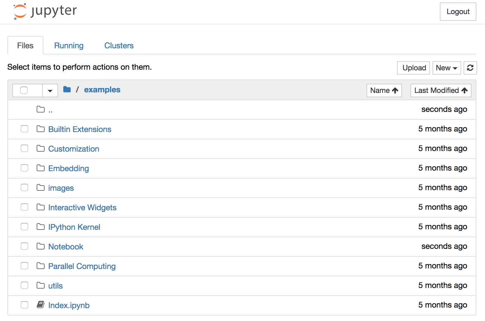
Files Tab
The files tab provides an interactive view of the portion of the filesystem which is accessible by the user. This is typically rooted by the directory in which the notebook server was started.
The top of the files list displays clickable breadcrumbs of the current directory. It is possible to navigate the filesystem by clicking on these breadcrumbs or on the directories displayed in the notebook list.
To create a new folder, click the New dropdown button and select Folder. New folder will be named Untitled Folder. Check the checkbox of the folder and click Rename button to rename folder.
A new python notebook can be created by clicking on the New dropdown button at the top of the list, and selecting Python 3 kernel.
Notebooks can also be uploaded to the current directory by clicking the Upload button at the top of the list.
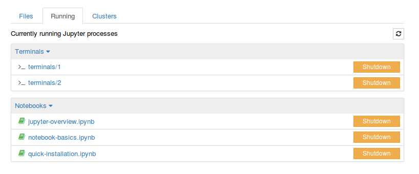
Running Tab
The running tab displays the currently running notebooks which are known to the server. This view provides a convenient way to track notebooks that have been started during a long running notebook server session.
Each running notebook will have an orange Shutdown button which can be used to shutdown its associated kernel. Closing the notebook’s page is not sufficient to shutdown a kernel.
Running terminals are also listed, provided that the notebook server is running on an operating system which supports PTY(Unix, Linux, Mac, but not Windows).
When there are too many running notebooks, you could encounter “Too many open files” error and all open notebooks will stop working properly. You can either restart the Jupyter server or click “shutdown” buttons in Running tab to reduce number of open notebooks. Just closing the notebook page won’t fix the issue.
The Notebook
When a notebook is opened, a new browser tab will be created which presents the notebook user interface (UI). This UI allows for interactively editing and running the notebook document.
A new notebook can be created from the dashboard by clicking on the Files tab, followed by the New dropdown button, and then selecting the language of choice(Python 3 for this course) for the notebook. From within a notebook, one can create a new python notebook by clicking File -> New Notebook -> Python 3 from the notebook menu bar.
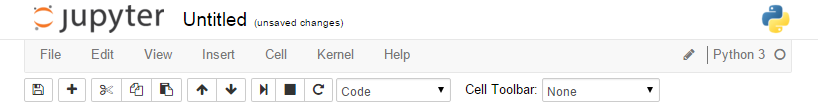
Header
At the top of the notebook document is a header which contains the notebook title, a menubar, and toolbar. This header remains fixed at the top of the screen, even as the body of the notebook is scrolled. The menubar and toolbar contain a variety of actions which control notebook navigation and document structure.
When a new notebook is created, the title will be Untitled. By clicking the title, it can be edited in-place (which renames the notebook file).
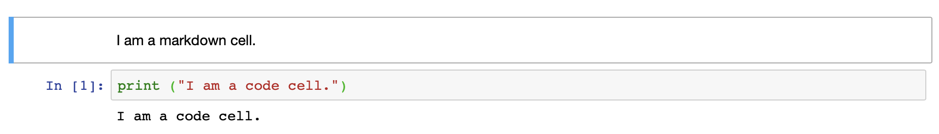
Body
The body of a notebook is composed of cells. Each cell contains either markdown, code input, code output, or raw text. Cells can be included in any order and edited at-will, allowing for a large amount of flexibility for constructing a narrative. We will only be using Code and Markdown cells in this course.
-
Markdown cells - These are used to build a nicely formatted narrative around the code in the document. The majority of this notebook is composed of markdown cells.
-
Code cells - These are used to define the computational code in the document. They come in two forms: the input cell where the user types the code to be executed, and the output cell which is the representation of the executed code. Depending on the code, this representation may be a simple scalar value, or something more complex like a plot or an interactive widget.
Cell Mode
The notebook user interface is modal. This means that the keyboard behaves differently depending upon the current mode of the notebook. A notebook cell has two modes: edit and command.
Edit mode is indicated by a green cell border and a prompt showing in the editor area. When a cell is in edit mode, you can type into the cell, like a normal text editor.

Command mode is indicated by a grey cell border. When in command mode, the structure of the notebook can be modified as a whole, but the text in individual cells cannot be changed. Most importantly, the keyboard is mapped to a set of shortcuts for efficiently performing notebook and cell actions. For example, pressing b when in command mode, will create a new cell below current cell.

Basic Workflow
Mouse Navigation
The first concept to understand in mouse-based navigation is that cells can be selected by clicking on them. The currently selected cell is indicated with a grey or green border depending on whether the notebook is in edit or command mode. Clicking inside a code cell’s editor area or double clicking a command cell will enter edit mode. Clicking on the prompt or the output area of a cell will enter command mode.
The second concept to understand in mouse-based navigation is that cell actions usually apply to the currently selected cell. For example, to run a code cell, select it and then click the button in the toolbar or the Cell -> Run menu item. Similarly, to change a code cell to markdown cell, click the drop down list in the tool bar and select Markdown or the Cell->Cell Type->Markdown. With this simple pattern, it should be possible to perform nearly every action with the mouse.
Markdown cells have one other state which can be modified with the mouse. These cells can either be rendered or unrendered. When they are rendered, a nice formatted representation of the cell’s contents will be presented. When they are unrendered, the raw text source of the cell will be presented. To render the selected cell with the mouse, click the button in the toolbar or the Cell -> Run menu item. To unrender the selected cell, double click on the cell.
Keyboard Navigation
All actions in the notebook can be performed with the mouse, but keyboard shortcuts are also available for the most common ones. This is made possible by having two different sets of keyboard shortcuts: one set that is active in edit mode and another in command mode. Click button in the tool bar for all keyboard shortcuts. The essential shortcuts to remember are the following:
- Esc: Command mode
- Enter: Edit mode
- Ctrl-Enter: Run cell
- Shift-Enter: Run cell and go to next cell
- Alt-Enter: Run cell and insert a new code cell below
- Under command mode
- a: Insert a new cell above
- b: Insert a new cell below
- dd: Delete cell. Caution:cannot undo delete
- y: Change cell to Code cell
- m: Change cell to Markdown cell
Magics
Jupyter provides specific commands, known as magics, that you can execute within a Code cell to provide enhanced functionality to the current notebook. Magics are not part of the Python programming language but can often make programming easier, especially within the notebook, and some magics can be used to improve your data processing work flow. Magics come in two types:
- line magics and
- cell magics.
To see the list of currently available magics, execute the following cell.
%lsmagic
Available line magics:
%alias  %alias_magic  %autoawait  %autocall  %automagic  %autosave  %bookmark  %cat  %cd  %clear  %colors  %config  %connect_info  %cp  %debug  %dhist  %dirs  %doctest_mode  %ed  %edit  %env  %gui  %hist  %history  %killbgscripts  %ldir  %less  %lf  %lk  %ll  %load  %load_ext  %loadpy  %logoff  %logon  %logstart  %logstate  %logstop  %ls  %lsmagic  %lx  %macro  %magic  %man  %matplotlib  %mkdir  %more  %mv  %notebook  %page  %pastebin  %pdb  %pdef  %pdoc  %pfile  %pinfo  %pinfo2  %popd  %pprint  %precision  %prun  %psearch  %psource  %pushd  %pwd  %pycat  %pylab  %qtconsole  %quickref  %recall  %rehashx  %reload_ext  %rep  %rerun  %reset  %reset_selective  %rm  %rmdir  %run  %save  %sc  %set_env  %store  %sx  %system  %tb  %time  %timeit  %unalias  %unload_ext  %who  %who_ls  %whos  %xdel  %xmode
Available cell magics:
%%!  %%HTML  %%SVG  %%bash  %%capture  %%debug  %%file  %%html  %%javascript  %%js  %%latex  %%markdown  %%perl  %%prun  %%pypy  %%python  %%python2  %%python3  %%ruby  %%script  %%sh  %%svg  %%sx  %%system  %%time  %%timeit  %%writefile
Automagic is ON, % prefix IS NOT needed for line magics.
Line magic
A line magic is prepended by a single % character and will have any arguments specified all on the same line. Some useful line magics include:
%lsmagic, which lists all currently defined line and cell magics for the current notebook,%matplotlib, which allows inline plotting to be enabled,%autosave, which sets the default autosave frequency in seconds, and%timeit, which in line mode times the execution of a single line of code.
Cell magics
A cell magic is prepended by two % characters and they can have arguments that include both the current line and the remaining lines in the current cell. Thus, cell magics must be placed on the first line of a cell, and in general you can only have one cell magic per cell. Some useful line magics include:
- ’%%timeit’, which can be used to time a multi-line Python statement,
- ’%%writefile’ writes the contents of the cell into the named file,
If you are uncertain how to use a particular magic, you can always obtain help from the notebook kernel by entering the magic by itself in a cell, adding a ? character at the end, and executing the cell to bring up the notebook help window.
Writing Markdown Document
Markdown is a plain text formatting syntax that you can easily use to write text that can be converted to formatted text, for example, HTML. Markdown was developed by John Gruber, who runs the popular [Daring Fireball][df] blog.
You can view the source of a markdown cell by double clicking on it, or while the cell is selected in command mode, press Enter to edit it. Use Shift-Enter to re-render a markdown cell when it is in edit mode. We will introduce markdown in more details in next lesson.
Writing and Executing Code
Of course, the reason we are using Jupyter Notebook is that it allows for in place development and execution of Python code. There are a number of direct benefits you accrue by developing and executing code in an Jupyter Notebook:
- Run code in place with the output displayed in the notebook,
- Display visualizations inline,
- Run code in the background, while you edit or run code in other cells,
- Clean restarts of the notebook kernel, and
- Built-in support for parallelization.
The simplest of these capabilities to demonstrate is developing and running code in the notebook. The code can be a single line or multiple lines. Code cells can be executed by using one of three key combinations: CONTROL-return, which executes the cell in place, SHIFT-return, which executes the code and advances to the next cell, or ALT-return, which executes the code and insert a new code cell below. For example, as shown below, we have a single line of Python code that can be executed with the output directly shown.
print("Hello World!")Hello World!
Key Points
Remember basic keyboard shortcuts
Be careful with command mode and edit mode